### DEGREE OF FLEXIBILITY... REGRESSION VS SMOOTH SPLINES ###

> setwd("C:/Users/baron/627 Statistical Machine Learning/data") 

> load("Auto.rda")

> attach(Auto)

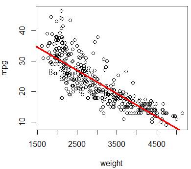
# Fit REGRESSION model predicting miles per gallon based on weight.

# Plot the regression line in red color with thickness=3

> reg = lm(mpg~weight)

> plot(weight,mpg)

> abline(reg,col="red",lwd=3)

# In general, abline(a,b) plots the line y = a + bx

# Fit a SPLINE with 2 degrees of freedom (straight line) to our data and plot it.

> spline2 = smooth.spline(weight,mpg,df=2)

> lines(spline2,col="blue")

# Add one more degree of freedom -> quadratic spline

> spline3 = smooth.spline(weight,mpg,df=3)

> lines(spline3,col="green",lwd=4)

# Increase flexibility by adding more d.f.

> spline20 = smooth.spline(weight,mpg,df=20)

> lines(spline20,col="brown",lwd=4)

# Blow flexibility to 100 degrees of freedom.

# The resulting spline is heavily dependent on each data point.

# Its prediction power is very low.

> spline100 = smooth.spline(weight,mpg,df=100)

> lines(spline100,col="orange",lwd=4)

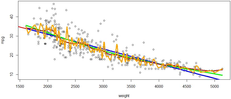
# While spline100 is very flexible, and it matches the data most closely, it would not be powerful for prediction. We’ll learn how to measure prediction accuracy with various cross-validation tools.

How to choose the optimal method? Cross-validation technique.

> n = length(mpg); Z = sample(n,n/2); attach(Auto[Z,]); # This will be our training data

> ss5 = smooth.spline(weight, mpg, df=5) # Fit the spline using training data only

> attach(Auto);

> Yhat = predict(ss5, x=weight)

> names(Yhat) # Notice: prediction consists of two parts – predictor x and

[1] "x" "y" # predicted response y. We can call them Yhat$x and Yhat$y.

> mean(( Yhat$y[-Z] - mpg[-Z] )^2) # Then, compute prediction mean-squared error on test data

[1] 17.76551 # This is the cross-validation error for a spline with df=5

# Try many different splines and choose the one with the smallest prediction error.

> cv.err = rep(0,50);

> for (p in 1:50){

+ attach(Auto[Z,]); ss = smooth.spline(weight, mpg, df=1+p/10) # Try DF = 1.1, 1.2, …, 6.0

+ attach(Auto); Yhat = predict(ss, weight) # DF must be > 1

+ cv.err[p] = mean( (Yhat$y[-Z] - mpg[-Z])^2 )

}

> df = 1+(1:50)/10

> plot(df,cv.err)

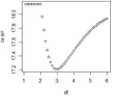
> which.min(cv.err)

[1] 20

> df[20]

[1] 3

# This cross-validation method chooses the spline with 3 d.f.